Anybody with even a passing interest in AI/ML likely knows the basics about neural networks. You connect a couple of layers of nodes with weights and biases, train it on some data, and bam, you've got a networik that can recognize cats or predict stock prices.

I always found this high-level understanding a little wishy-washy, though. Even when working through Kaggle courses over the summer, fully building out these models in Tensorflow, I felt like I didn't understand what was going on or what I should be paying attention to in the code.

I didn't start building this intuition until taking Andrew Ng's Intro to ML course on Coursera, which taught ML principles and algorithms not using Tensorflow or Keras — the course assignments used Matlab — but through the underlying math and equations that make these models tick. For me, this concrete technical understanding was a huge boost for my understanding of ML overall. I visualized gradient descent for a simple linear regression model in a blog post two months ago. To further solidify my learning, I spent a few hours in the past few days building a simple neural network from scratch, and trained it to recognize handwritten digits from the MNIST dataset.

In this blog post, I'll be giving an explanation of the math behind neural networks, and a walkthrough of how I implemented it using numpy.

---

If you just want to see the code and don't need a ton of explanation, have a look at my Kaggle notebook for the project.

---

Problem Statement

The dataset we're working with is the famous MNIST handwritten digit dataset, commonly used for instructive ML and computer vision projects. It contains 28 x 28 grayscale images of handwritten digits that look like this:

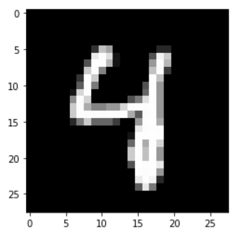
Each image is accompanied by a label of what digit it belongs to, from 0 to 9. Our task is to build a network that takes in an image like this and predicts what digit is written in it.

Neural Network Overview

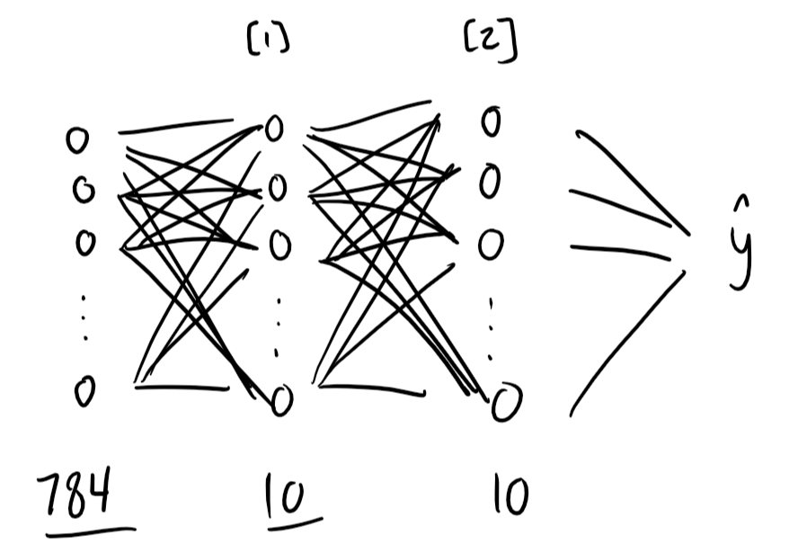
Our network will have three layers total: an input layer and two layers with parameters. Because the input layer has no parameters, this network would be referred to as a two-layer neural network.

The input layer has 784 nodes, corresponding to each of the 784 pixels in the 28x28 input image. Each pixel has a value between 0 and 255, with 0 being black and 255 being white. It's common to normalize these values — getting all values between 0 and 1, here by simply dividing by 255 — before feeding them in the network.

The second layer, or hidden layer, could have any amount of nodes, but we've made it really simple here with just 10 nodes. The value of each of these nodes is calculated based on weights and biases applied to the value of the 784 nodes in the input layer. After this calculation, a ReLU activation is applied to all nodes in the layer (more on this later).

In a deeper network, there may be multiple hidden layers back to back before the output layer. In this network, we'll only have one hidden layer before going to the output.

The output layer also has 10 nodes, corresponding to each of the output classes (digits 0 to 9). The value of each of these nodes will again be calculated from weights and biases applied to the value of the 10 nodes in the hidden layer, with a softmax activation applied to them to get the final output.

The process of taking an image input and running through the neural network to get a prediction is called forward propagation. The prediction that is made from a given image depends on the weights and biases, or parameters, of the network.

To train a neural network, then, we need to update these weights and biases to produce accurate predictions. We do this through a process called gradient descent. The basic idea of gradient descent is to figure out what direction each parameter can go in to decrease error by the greatest amount, then nudge each parameter in its corresponding direction over and over again until the parameters for minimum error and highest accuracy are found. Check out my visualization of gradient descent here.

In a neural network, gradient descent is carried out via a process called backward propagation, or backprop. In backprop, instead of taking an input image and running it forwards through the network to get a prediction, we take the previously made prediction, calculate an error of how off it was from the actual value, then run this error backwards through the network to find out how much each weight and bias parameter contributed to this error. Once we have these error derivative terms, we can nudge our weights and biases accordingly to improve our model. Do it enough times, and we'll have a neural network that can recognize handwritten digits accurately.

The Math

That's the high level overview — now let's get into the math. This section contains quite a lot of matrix/vector operations, and just a little calculus, so be prepared!

Representing our data

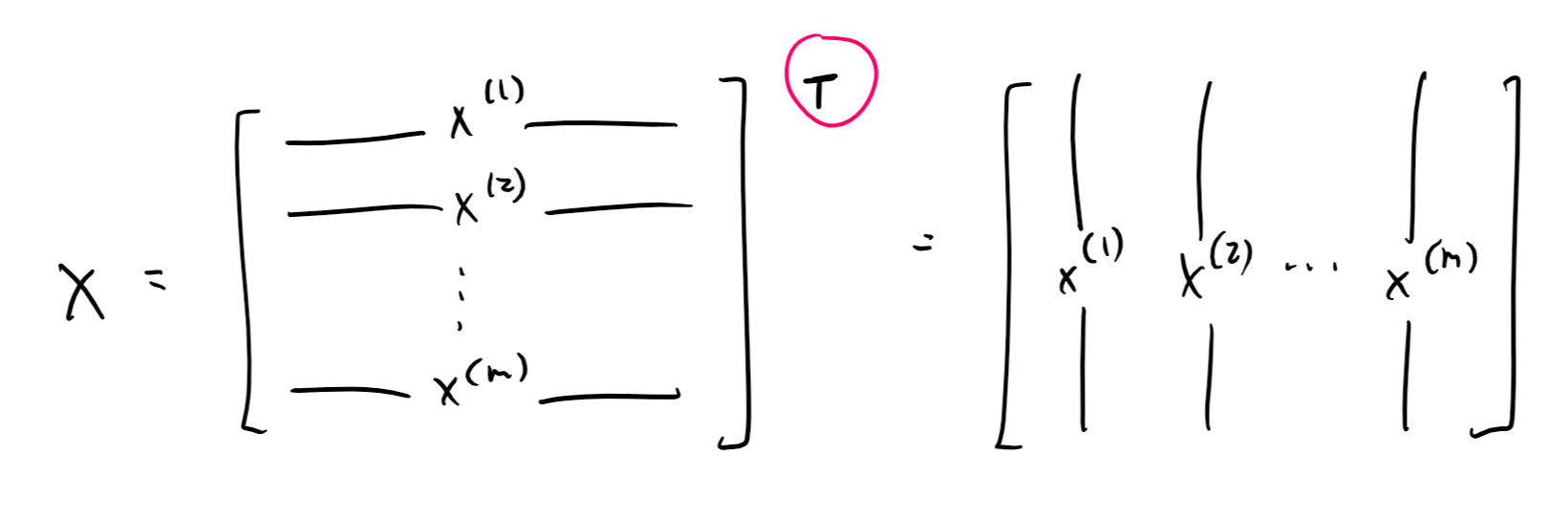
As mentioned earlier, each training example can be represented by a vector with 784 elements, corresponding to each of the image's 784 pixels.

These vectors can be stacked together in a matrix to carry out vectorized calculations. That is, instead of using a for loop to go over all training examples, we can calculate error from all examples at once with matrix operations.

In most contexts, including for machine learning, the convention is to stack these vectors as rows of the matrix, giving the matrix dimensions of $$m : \text{rows} \times n : \text{columns}$$, where $$m$$ is the number of training examples and $$n$$ is the number of features, in this case 784. To make our math easier, we're going to transpose this matrix, giving it dimensions $$n \times m$$ instead, with each column corresponding to a training example and each row a training feature.

Representing weights and biases

Let's look at our neural network now. Between every two layers is a set of connections between every node in the previous layer and every node in the following one. That is, there is a weight $$w_{i,j}$$ for every $$i$$ in the number of nodes in the previous layer and every $$j$$ in the number of nodes in the following one.

It's natural, then, to represent our weights as a matrix of dimensions $$n^{[l]}\times n^{[l-1]}$$, where $$n^{[l-1]}$$ is the number of nodes in the previous layer and $$n^{[l]}$$is the number of nodes in the following layer. Let's call this matrix $$W^{[l]}$$, corresponding to layer $$l$$ of our network. $$W^{[1]}$$, for example, will be a $$10\times784$$ matrix, taking us from the 784 nodes of the input layer to the 10 nodes of the first hidden layer. $$W^{[2]}$$ will have dimensions $$10\times10$$.

Biases are simply constant terms added to each node of the following layer, so we can represent it as a matrix with dimensions $$n^{[l]}\times 1$$. Let's call these matrices $$b^{[l]}$$, so that $$b^{[1]}$$ and $$b^{[2]}$$ both have dimensions $$10\times1$$.

Forward propagation

With these representations in mind, we can now write the equations for forward propagation.

First, we'll compute the unactivated values of the nodes in the first hidden layer by applying $$W^{[1]}$$ and $$b^{[1]}$$ to our input layer. We'll call the output of this operation $$Z^{[1]}$$:

$$Z^{[1]} = W^{[1]}X+b^{[1]}$$

Remember that $$X$$ has dimensions $$784\times m$$, and $$W^{[1]} : 10\times784$$. $$W^{[1]}X$$ is the dot product between the two, yielding a new matrix of dimensions $$10\times m$$. This may seem a little strange at first, but think of it this way: each column of this matrix corresponds to the unactivated values for the nodes in the first hidden layer when carried out for one training example, so the entire matrix represents carrying out the first step of forward propagation for all training examples at the same time. This is much more efficient than a for loop, and is what was referred to earlier as a "vectorized implementation."

Our bias term $$b^{[1]}$$has dimensions $$10\times1$$, but we want the same column of biases to be applied to all $$m$$ columns of training examples, so $$b^{[1]}$$is effectively broadcast into a matrix of dimensions $$10\times m$$ when calculating $$Z^{[1]}$$, matching the dimensions of $$W^{[1]}X$$.

We need to do one more calculation before moving on to the next layer, though, and that's applying a non-linear activation to $$Z^{[1]}$$. What does this mean, and why do we have to do it?

Imagine that we didn't do anything to $$Z^{[1]}$$ now, and multiplied it by $$W^{[2]}$$ and added $$b^{[2]}$$ to get the value for the next layer. $$Z^{[1]}$$ is a linear combination of the input features, and the second layer would be a linear combination of $$Z^{[1]}$$, making it still a linear combination of the input features. That means that our hidden layer is essentially useless, and we're just building a linear regression model.

To prevent this reduction and actually add complexity with our layers, we'll run $$Z^{[1]}$$ through a non-linear activation function before passing it off to the next layer. In this case, we'll be using a function called a rectified linear unit, or ReLU:

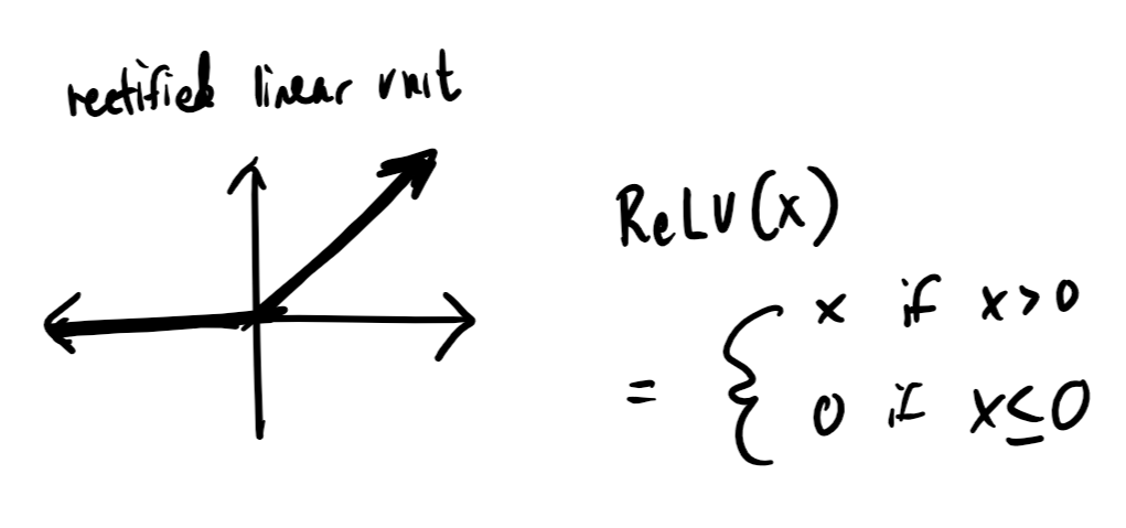
ReLU is a really simple function: it's linear if the input value is above 0, and outputs 0 otherwise. Just this much, though, is enough to ensure that our model doesn't collapse to a linear one.

From $$Z^{[1]}$$, we'll calculate a value $$A^{[1]}$$ for the values of the nodes in the hidden layer of our neural network after applying our activation function to it:

$$A^{[1]} = \text{ReLU}(Z^{[1]})$$

More generally, you might see this written as $$A^{[l]} = g(Z^{[l]})$$, with $$g$$ referring to an arbitrary activation function that may be something other than ReLU.

Once we have $$A^{[1]}$$, we can proceed to calculating the values for our second layer, which is also our output layer. First, we calculate $$Z^{[2]}$$:

$$Z^{[2]} = W^{[2]}A^{[1]}+b^{[2]}$$

Then, we'll apply an activation function to $$Z^{[2]}$$ to get our final output.

If this second layer were just another hidden layer, with more hidden layers or an output layer after it, we would apply ReLU again. But since it's the output layer, we'll apply a special activation function called softmax:

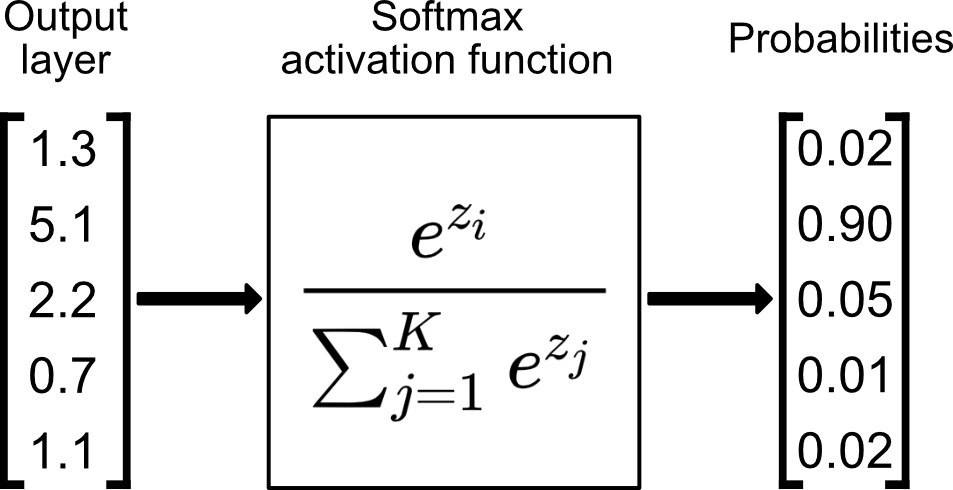
Diagram by Bartosz Szabłowski on Towards Data Science

Softmax takes a column of data at a time, taking each element in the column and outputting the exponential of that element divided by the sum of the exponentials of each of the elements in the input column. The end result is a column of probabilities between 0 and 1.

The value of using softmax for our output layer is that we can read the output as probabilities for certain predictions. In the diagram above, for example, we might read the output as a prediction that the second class has a 90% probability of being the correct label, the third a 5% probability, the fourth a 1% probability, and so on.

Let's find our $$A^{[2]}$$:

$$A^{[2]} = \text{softmax}(Z^{[2]})$$

Softmax runs element-wise, so the dimensions of $$Z^{[2]}$$ are preserved at $$10\times m$$. We can read this output matrix as follows: value $$A^{[2]}_{i, j}$$ is the probability that example $$j$$ is an image of the digit $$i$$.

With that, we've run through the entire neural network, going from our input $$X$$ containing all of our training examples to an output matrix $$A^{[2]}$$ containing prediction probabilities for each example.

Backward propagation

Now, we'll go the opposite way and calculate how to nudge our parameters to carry out gradient descent.

Mathematically, what we're actually computing is the derivative of the loss function with respect to each weight and bias parameter. For a softmax classifier, we'll use a cross-entropy loss function:

$$J(\hat{y}, y) = -\sum_{i=0}^{c} y_i \log(\hat{y}_i)$$

Here, $$\hat{y}$$ is our prediction vector. It might look like this:

$$\begin{bmatrix} 0.01 \ 0.02 \ 0.05 \ 0.02 \ 0.80 \ 0.01 \ 0.01 \ 0.00 \ 0.01 \ 0.07 \ \end{bmatrix}$$

$$y$$ is the one-hot encoding of the correct label for the training example. If the label for a training example is 4, for example, the one-hot encoding of $$y$$ would look like this:

$$\begin{bmatrix} 0 \ 0 \ 0 \ 0 \ 1 \ 0 \ 0 \ 0 \ 0 \ 0 \ \end{bmatrix}$$

Notice that in our sum $$\sum_{i=0}^{c} y_i \log(\hat{y}_i)$$, $$y_i = 0$$ for all $$i$$ except the correct label. The loss for a given example, then, is just the log of the probability given for the correct prediction. In our example above, $$J(\hat{y}, y) = -\log(y_4) = -\log(0.80) \approx 0.097$$. Notice that, the closer the prediction probability is to 1, the closer the loss is to 0. As the probability approaches 0, the loss approaches $$+\infty$$. By minimizing the cost function, we improve the accuracy of our model. We do so by substracting the derivative of the loss function with respect to each parameter from that parameter over many rounds of graident descent:

$$W^{[1]} := W^{[1]} - \alpha \frac{\delta J}{\delta W^{[1]}} \ b^{[1]} := b^{[1]} - \alpha \frac{\delta J}{\delta b^{[1]}} \ W^{[2]} := W^{[2]} - \alpha \frac{\delta J}{\delta W^{[2]}} \ b^{[2]} := b^{[2]} - \alpha \frac{\delta J}{\delta b^{[2]}} \ $$

Our objective in backprop is to find $$\frac{\delta J}{\delta W^{[1]}},\frac{\delta J}{\delta b^{[1]}},\frac{\delta J}{\delta W^{[2]}},$$ and $$\frac{\delta J}{\delta b^{[2]}}$$. For concision, we'll write these values as $$dW^{[1]}, db^{[1]}, dW^{[2]},$$and $$db^{[2]}$$. We'll find these values by stepping backwards through our network, starting by calculating $$\frac{\delta J}{\delta A^{[2]}}$$, or $$dA^{[2]}$$. Turns out that this derivative is simply:

$$dA^{[2]} = Y - A^{[2]}$$

If you know calculus, you can take the derivative of the loss function and confirm this for yourself. (Hint: $$\hat{y} = A^{[2]}$$)

From $$dA^{[2]}$$, we can calculate $$dW^{[2]}$$ and $$db^{[1]}$$:

$$dW^{[2]} = \frac{1}{m} dZ^{[2]} A^{[1]T} \ dB^{[2]} = \frac{1}{m} \Sigma {dZ^{[2]}}$$

Then, to calculate $$dW^{[1]}$$ and $$db^{[1]}$$, we'll first find $$dZ^{[1]}$$:

$$dZ^{[1]} = W^{[2]T} dZ^{[2]} .* g^{[1]\prime} (Z^{[1]})$$

I won't explain all the details of the math, but you can get some intuitive hints at what's going on here by just looking at the variables. We're applying $$W^{[2]T}$$ to $$dZ^{[2]}$$, akin to applying the weights between layers 1 and 2 in reverse. Then, we perform an element-wise multiplication with the derivative of the activation function, akin to "undoing" it to get the correct error values.

Since our activation function is ReLU, our derivative is actually pretty simple. Let's revisit our graph:

When the input value is greater than 0, the activation function is linear with a derivative of 1. When the input value is less than 0, the activation function is horizontal with a derivative of 0. Thus, $$g^{[1]\prime}(Z^{[1]})$$ is just a matrix of 1s and 0s based on values of $$Z^{[1]}$$.

From here, we do the same calculations as earlier to find $$dW^{[1]}$$ and $$db^{[1]}$$, using $$X$$ in place of $$A^{[1]}$$:

$$dW^{[1]} = \frac{1}{m} dZ^{[1]} X^T \ dB^{[1]} = \frac{1}{m} \Sigma {dZ^{[1]}}$$

Now we've found all the derivatives we need, and all that's left is to update our parameters:

$$W^{[2]} := W^{[2]} - \alpha dW^{[2]} \ b^{[2]} := b^{[2]} - \alpha db^{[2]} \ W^{[1]} := W^{[1]} - \alpha dW^{[1]} \ b^{[1]} := b^{[1]} - \alpha db^{[1]}$$

Here, $$\alpha$$is our learning rate, a "hyperparameter" that we set to whatever we want. $$\alpha$$ is distinguished from other parameters because, just like the number of layers in the network or the number of units in each layer, it's a value that we choose for our model rather than one that gradient descent optimizes.

With that, we've gone over all the math that we need to carry out gradient descent and train our neural network. To recap: first, we carry out forward propagation, getting a prediction from an input image:

$$Z^{[1]} = W^{[1]} X + b^{[1]}\A^{[1]} = g_{\text{ReLU}}(Z^{[1]}))\Z^{[2]} = W^{[2]} A^{[1]} + b^{[2]}\A^{[2]} = g_{\text{softmax}}(Z^{[2]})$$

Then, we carry out backprop to compute loss function derivatives:

$$dZ^{[2]} = A^{[2]} - Y\dW^{[2]} = \frac{1}{m} dZ^{[2]} A^{[1]T}\dB^{[2]} = \frac{1}{m} \Sigma {dZ^{[2]}}\dZ^{[1]} = W^{[2]T} dZ^{[2]} .* g^{[1]\prime} (z^{[1]})\dW^{[1]} = \frac{1}{m} dZ^{[1]} A^{[0]T}\dB^{[1]} = \frac{1}{m} \Sigma {dZ^{[1]}}$$

Finally, we update our parameters accordingly:

$$W^{[2]} := W^{[2]} - \alpha dW^{[2]} \ b^{[2]} := b^{[2]} - \alpha db^{[2]} \ W^{[1]} := W^{[1]} - \alpha dW^{[1]} \ b^{[1]} := b^{[1]} - \alpha db^{[1]}$$

We'll do this process over and over again — the exact number of times, an iteration count that we again set ourselves — until we are satisfied with the performance of our model.

The code

With all the math out of the way, all that's left is to implement our neural network in code. I did so in a Python Jupyter notebook hosted on Kaggle — you can see all my code here: https://www.kaggle.com/wwsalmon/simple-mnist-nn-from-scratch-numpy-no-tf-keras

First, we'll import numpy to help us manipulate our data matrices and carry out linear algebra operations. (In the Kaggle notebook I also import pandas to help with reading in data and matplotlib to display images).

import numpy as np

We'll then initialize our parameters to matrices of small, random values of the correct shape:

def init_params():
    W1 = np.random.rand(10, 784) - 0.5
    b1 = np.random.rand(10, 1) - 0.5
    W2 = np.random.rand(10, 10) - 0.5
    b2 = np.random.rand(10, 1) - 0.5
    return W1, b1, W2, b2

With parameters and matrix $$X$$as input, we can write a function to carry out forward propagation:

def forward_prop(W1, b1, W2, b2, X):
    Z1 = W1.dot(X) + b1
    A1 = ReLU(Z1)
    Z2 = W2.dot(A1) + b2
    A2 = softmax(Z2)
    return Z1, A1, Z2, A2

We'll need to fill in two helper functions here for our two activation functions:

def ReLU(Z):
    return np.maximum(Z, 0)

def softmax(Z):
    return np.exp(Z) / sum(np.exp(Z))

Notice that we returned not just our final predictions but also Z1, A2, and Z2 from our forward prop function. This is because we'll now pass them into a backprop function:

def backward_prop(Z1, A1, Z2, A2, W1, W2, X, Y):
    one_hot_Y = one_hot(Y)
    dZ2 = A2 - one_hot_Y
    dW2 = 1 / m * dZ2.dot(A1.T)
    db2 = 1 / m * np.sum(dZ2)
    dZ1 = W2.T.dot(dZ2) * ReLU_deriv(Z1)
    dW1 = 1 / m * dZ1.dot(X.T)
    db1 = 1 / m * np.sum(dZ1)
    return dW1, db1, dW2, db2

Again, we'll need some helper functions for the derivative of our ReLU activation function and for one-hot encoding of our labels Y:

def ReLU_deriv(Z):
    return Z > 0

def one_hot(Y):
    one_hot_Y = np.zeros((Y.size, Y.max() + 1))
    one_hot_Y[np.arange(Y.size), Y] = 1
    one_hot_Y = one_hot_Y.T
    return one_hot_Y

Finally, once we have our derivative values, we complete gradient descent by updating our parameters.

def update_params(W1, b1, W2, b2, dW1, db1, dW2, db2, alpha):
    W1 = W1 - alpha * dW1
    b1 = b1 - alpha * db1    
    W2 = W2 - alpha * dW2  
    b2 = b2 - alpha * db2    
    return W1, b1, W2, b2

We'll tie it all together with a for loop in a wrapper function, with another two helper functions for printing out the accuracy on every 10th iteration:

def get_predictions(A2):
    return np.argmax(A2, 0)

def get_accuracy(predictions, Y):
    print(predictions, Y)
    return np.sum(predictions == Y) / Y.size

def gradient_descent(X, Y, alpha, iterations):
    W1, b1, W2, b2 = init_params()
    for i in range(iterations):
        Z1, A1, Z2, A2 = forward_prop(W1, b1, W2, b2, X)
        dW1, db1, dW2, db2 = backward_prop(Z1, A1, Z2, A2, W1, W2, X, Y)
        W1, b1, W2, b2 = update_params(W1, b1, W2, b2, dW1, db1, dW2, db2, alpha)
        if i % 10 == 0:
            print("Iteration: ", i)
            predictions = get_predictions(A2)
            print(get_accuracy(predictions, Y))
    return W1, b1, W2, b2

With that, we can run our gradient_descent function on our training X and Y data, as well as learning rate alpha and number of iterations iterations, to get trained parameters W1, b1, W2, and b2:

W1, b1, W2, b2 = gradient_descent(X_train, Y_train, 0.10, 500)

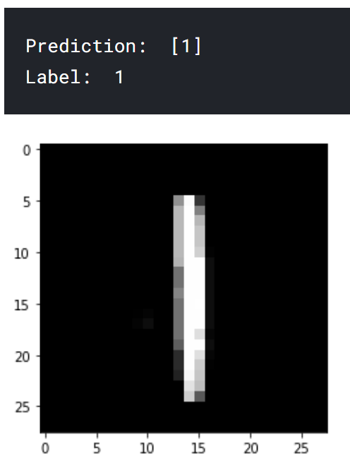
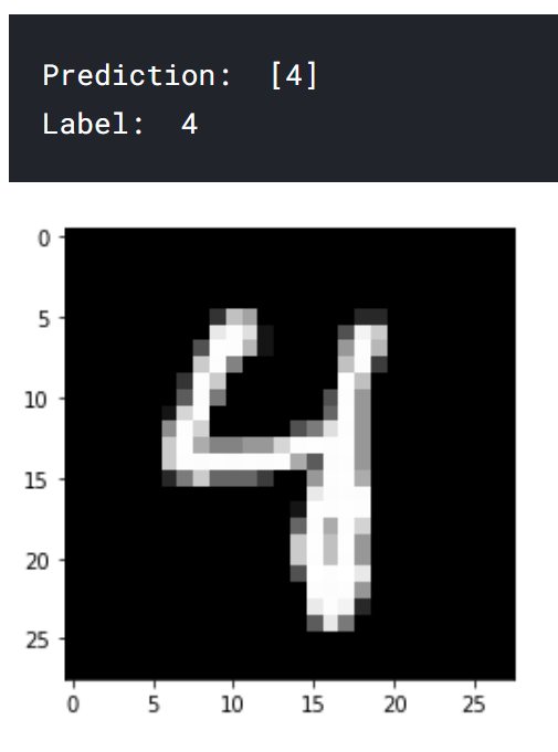
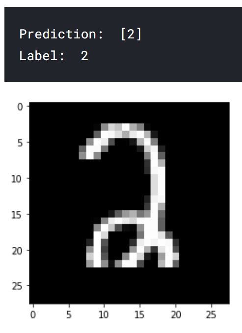
In the Kaggle notebook, with a training dataset of 41,000 examples, this model achieved an accuracy of 85% on the training data, and 84% on 1,000 examples set aside as test data.

A few prediction examples:

Conclusion

And that's it! We've run through all the math behind how a neural network works, and implemented it in Python, training a real model with an 84% accuracy when identifying handwritten images.

There are many ways that this model could be improved. The dataset is a fairly easy one to build a model for, with top solutions hitting above 99% accuracy. Even before considering fancy architectures like CNNs, just adding more hidden layers or units to our model would help it recognize patterns and make predictions more effectively.

There are many possible optimizations for the gradient descent process, too. Gradient descent with momentum, RMSProp, and Adam optimization are popular variations of gradient descent that improve training efficiency.

Of course, it doesn't make sense to go out and code super-complex models yourself when frameworks like Tensorflow have already implemented them and tons of other optimizations and functionality. The purpose of this neural network from scratch project was to be instructive, providing an in-depth walkthrough not just of how a neural network works in theory, but into the intricacies of the math and code that make it tick. You'll rarely use this knowledge directly in further machine learning application or learning, but at least to me, it's a path to building a solid foundation from which more advanced exploration can launch.

I hope that some of you will find this article helpful! Once again, you can find the Kaggle notebook with all my code here, and a video walkthrough of everything in this article here.

If you want to follow along with my projects and learning, subscribe to my newsletter here!