If you've taken a lab science class in school, you've probably had to fit a line of best fit to experimental data: whether it's to experimentally determine the acceleration of gravity, calculate the results of a chemical reaction, or prove that two variables are correlated. You plug your numbers into a spreadsheet, hit "fit trendline," and out pops a nice linear or exponential equation. But how does Excel or Google Sheets come up with this equation?

This problem is that of training a linear regression model. There are lots of statistics-related theorems and considerations behind it, but this article will focus on an algorithm that computers use to actually find the best fit equation given a dataset. The same principles that empower Excel to find a line of best fit are the fundamentals for a variety of machine learning algorithms and applications, from deep neural networks to recommendation systems. Understanding linear regression is a great first step to understanding all the other cool ML algorithms out there — and it's not even that hard! Let's dive in.

Note: all graphs, calculations, and even data used in this article were created by me in Python. Check out the source code in this Jupyter notebook.

The basics: mean squared error cost function

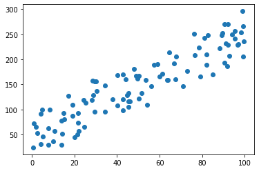
Here's a dataset to fit a line to.

If you've taken Algebra, you should be familiar with the equation for a line:

$$y = mx + b$$

By tweaking m and b, we can conjure up any line that we want to. We can take a few guesses at a line of best fit for our dataset:

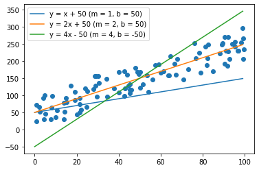
Clearly, some of these lines fit the data better than others. Yellow looks the best — green is too steep, and blue isn't steep enough. But how can we know for sure that yellow is better than green and blue? And how can we find not just a good line, but the best line possible?

We can start by coming up with a number to measure how well a line fits the given data. We can use a metric called the mean squared error.

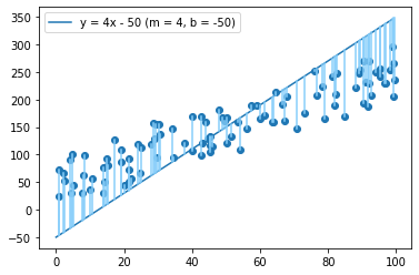
To calculate the mean squared error, take every example and measure the vertical distance between it and the line above or below. Square this distance, then average the squares of all examples.

Here's the formula for calculating mean squared error for our linear equation:

{% raw %} $$J = \frac{1}{2 \cdot \text{# examples}} \sum_{i = 1}^\text{# examples} ((mx^{(i)}+b) - y^{(i)})^2$$ {% endraw %}

where $$x^{(i)}$$ and $$y^{(i)}$$ are the i-th pair of x and y values in our dataset.

The lower the MSE is, the better the line fits the data. This should make sense — all that MSE is measuring is the average squared distance from the data points to the corresponding predicted value on the line. The smaller this distance, the better the line.

We can use a simple loop in Python to calculate the mean squared error of the three lines we guessed above:

def mean_squared_error(m, b, x_data, y_data):
	num_examples = x_data.size
	J = 0

	for i in range(num_examples):
		J += ((m * x_data[i] + b) - y_data[i]) ** 2

	J = J / (2 * num_examples)

	return J

print(mean_squared_error(1, 50, x_data, y_data))
print(mean_squared_error(2, 50, x_data, y_data))
print(mean_squared_error(4, -50, x_data, y_data))

We get that the MSE for the first line — our blue, too low line — is 2070.76. The MSE for the second line — our yellow, seems-best line — is a mere 375.26. The MSE for the third line — the green, too-steep line — is back up to 2280.60.

This confirms our visual findings from before. Our yellow line, with the equation $$y = 2x + 50$$, has the lowest MSE and fits the data much better than the two other lines. By this metric, our blue line is also worse than our green line.

With this metric, we're one step closer to a systematic way to find a line of best fit. We can now guess a bunch of lines, and then check their mean squared error, keeping the one with the lowest MSE and maybe tweaking it some more.

This is random and inefficient, though. Luckily, there's a much better, systematic way of finding the best possible line once we've defined our cost function (MSE).

Finding the optimal solution: gradient descent

Let's return to one of our bad lines:

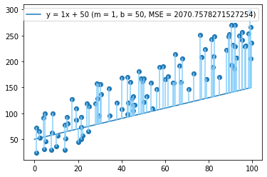
If we want to improve it, what should we do? A lot of the points look like they're above the line, so let's increase b to 70.

Looks a little better, and our MSE has dropped by almost 40%, from 2071 to 1286! Let's keep going and increase b to 90.

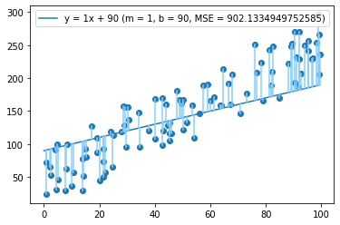
Another drop, to MSE = 902. Now let's try b = 110:

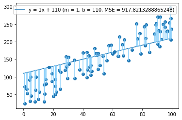
...and now we've overshot it, with our MSE increasing to 918.

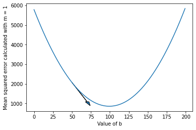
To find the optimal value of b and not overshoot, we might graph the MSE against different values of b.

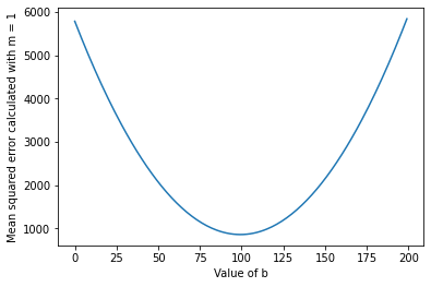
Looks like the optimal value is just below 100. If you've taken algebra or calculus, your instinct at this point might be to bust out some derivatives or quadratic equations and try to find out exactly what this point is — but it's not so easy, because we don't actually have the equation for this line. Every one of those points above was computed by looping through 100 training examples and averaging their errors.

Instead of finding the optimal value analytically, then, we do it numerically.¹ These are fancy names for saying that instead of trying to solve an equation exactly, we'll use clever tricks to arrive at the right answer by changing our answers just a little bit, over and over.

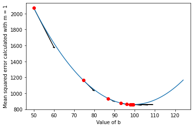
Let's go back to our starting point at b = 50. Let's plot the slope of our b vs. MSE plot at b = 50:

We can find the slope at a given point using this formula:

$$\frac{\delta J}{\delta b} = \frac{1}{\text{# examples}} \sum_{i = 1}^\text{# examples} ((mx^{(i)}+b) - y^{(i)})$$

If you've taken calculus, you can take the derivative of our earlier mean squared error function (J) with respect to b yourself and see if your answer matches. If you don't know calculus, just accept that this equation accurately gives us the slope at a given point. Look into derivatives separately if you want.

The point is, once we have this slope, we can nudge b an amount proportional to the steepness of the slope. Think of it like rolling down a hill. If the hill is steeper, you'll roll down more. If it's shallower, you'll roll down less. If you keep rolling down a hill like this, you'll eventually get to the lowest point of the valley — and in this case, our ideal value for b.

In equation form, this is what we're doing:

$$\text{repeat } i \text{ times } {

b := b - \alpha \frac{\delta J}{\delta b}

}$$

It might look a little confusing, but all we're doing here is what we said earlier: nudging b an amount proportional to the steepness, or gradient, of the graph of the cost function at that point. $$\alpha$$, or alpha, is called the "learning rate" — it's a multiplier on how much you slide down the hill, something like the strength of gravity or the slipperiness of the hill. If alpha is big, you'll slide down the hill quickly. If it's small, you'll slide down it bit by bit. As you slide towards the bottom of the valley, the gradient will flatten out and steps will become smaller. The value that you're optimizing will then converge to the value that results in the lowest error — the best fit b for your data, in this case.

With a learning rate of 0.5, we roughly converge to a b value around 99 in less than ten steps:

We've only found the optimal value for b, however. Our MSE is still above 800, more than double that of our initial best-guess line, 2x + 50. We could now set b to be 99 and optimize for m, but that wouldn't get us the best answer either. To get the actual line of best fit, we have to optimize for both m and b at the same time.

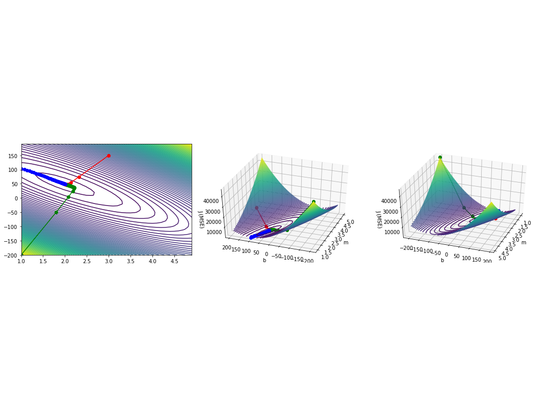
To do this, we can plot J against both m and b using a contour map:

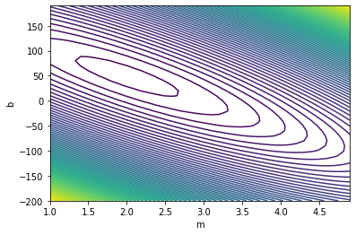
You may have seen contour maps of a mountain or particular region before. Such a map shows the land elevation at a given point. The contour map above does a very similar thing: it shows the mean squared error for every pair of $$m$$ and $$b$$ values. By finding the $$m$$ and $$b$$ values that give us the lowest possible mean squared error, then, we'll have found our line of best fit.

The intuition here — and the math — is the same as before: we find the slope (gradient) at a given point, and roll down the hill (change our parameters) an amount proportional to how steep the slope is. When we calculate the gradient at a certain point, we no longer have just one value, but two values, corresponding to how the cost function changes when you nudge either m or b.

The formula for calculating these two gradient values at a given point are as follows:

$$\frac{\delta J}{\delta b} = \frac{1}{\text{# examples}}\sum_{i = 1}^\text{# examples} ((mx^{(i)}+b) - y^{(i)}) \ \frac{\delta J}{\delta m} = \frac{1}{\text{# examples}}\sum_{i = 1}^\text{# examples} ((mx^{(i)}+b) - y^{(i)})x$$

Before, we subtracted the gradient with respect to b, times a learning rate, from b to get our new value. We'll do that again here, and we'll do the same separately for m, at the same time:

$$\text{repeat } i \text{ times }\{\ b := b - \alpha \frac{\delta J}{\delta b} \ m := m - \alpha \frac{\delta J}{\delta m} \}$$

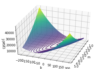
Just as before, we can illustrate this two-variable gradient descent visually on our contour map and 3D plot. I plotted gradient descent from three starting points (red: m = 3, b = 150; green: m = 1, b = -200; blue: m = 1, b = 103).

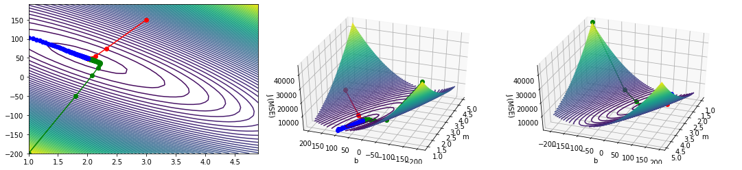
As you can see, it doesn't matter where you start — gradient descent will eventually lead you to the right answer. In fact, standard practice when training machine learning models is to use small random values for your starting points.

In this case, following the gradient, we find an approximate global minimum at m = 2 and b = 49. Translating back from the world of equations and graphs, this means that the line (approximately) $$y = 2x + 49$$ results in the lowest mean squared error when measured against our dataset, and consequently is the line of best fit for the dataset², what we've been looking for all along.

Phew! After all that hard work, we're finally done. Let's do a quick recap of what just went down.

• We defined a cost function, something called the "mean squared error" that measures how far the predictions of our model are from the actual data.
• Our objective is to minimize the cost function (in fact, another name for the cost function is the "objective function").
• We started this by graphing the cost function against one parameter, in this case the y-intercept (b) of the line.
• To minimize the cost function, we "nudged" the parameter in the direction that would decrease the cost.
• We used gradient descent is a way to make these nudges systematically, by choosing them proportional to the slope, or gradient, of the graph. It's like rolling downhill!
• We then included our second parameter, in this case the slope of the line, in our graph of the cost function. It can now be visualized as a contour plot, or a 3D surface.
• We can apply the same method as earlier — gradient descent, sliding downhill with the slope of the 3D surface — to optimize both parameters at once. This gives us the optimal parameters m and b, yielding our line of best fit.

This might seem like a lot to take in, especially the mathematical equations. I know it took me a good few learning days to gain a sense of comfort with them. Understanding the math behind how to fit a trendline, though, is incredibly useful for understanding tons of other machine learning algorithms out there.

Beyond linear regression: a fundamental concept in machine learning

The general pattern of defining a cost function and using gradient descent to optimize for it is ubiquitous in supervised learning algorithms. Fitting a polynomial function to a dataset rather than a straight line, for example, is as easy as defining the cost function as the following:

$$J = \frac{1}{2 \cdot \text{# examples}} \sum_{i = 1}^\text{# examples} ((\theta_0 + \theta_1 x^{(i)} + \theta_2 x^{(i)2}) - y^{(i)})^2$$

where we now have three parameters theta 0, theta 1, and theta 2 to optimize rather than just m and b. In fact, we can throw as many more parameters as we want at the cost function, and very often optimize hundreds or thousands of parameters in just this way.

Instead of a line of best fit (a regression model with continuous outputs), we can train a classifier using the very same cost function-gradient descent strategy. We do this by running the continuous model output through a logistic (or sigmoid) function, which outputs a number between 0 and 1 that we can interpret as a probability of the input belonging to a certain class.

Neural networks use cost functions and gradient descent too, though the cost function and parameter optimization methods are a bit more complicated, involving in-between feed-forward and backpropagation algorithms.

Even some unsupervised learning problems — that is, models where there is no "right" answer that can be provided in training data — use cost functions and gradient descent. When training a recommendation algorithm, like Netflix or Amazon might use to recommend you movies and products, a cost function is defined that simultaneously optimizes for parameters fitting users' preferences and the categorization of different items.

It's easy to just say these things. You might even have heard of gradient descent, and the analogy of sliding down a hill, before reading this article. For me at least, though, it's much more helpful to see the concrete math. I like learning how an algorithm works well enough to be able to code it from scratch, without using TensorFlow or scikit-learn or whatever is out there. Of course, if I'm working on an actual project, I'll use the better-optimized and more advanced tools that these libraries have to offer; even then, though, I'm guided by the intuition I gained from going very hands-on into the math.

A lot of the math isn't super hard, either. In this article, for example, the most advanced things that you need to understand are summation loops and...squares. Sure, there were a few derivatives, but I didn't tell you what they meant, because you don't need to know to build your core mathematical machine learning intuition. This relative mathematical simplicity extends, again, beyond linear regression to most of the common machine learning algorithms in use out there. Neural networks are really just a lot of summation loops strung together cleverly. If you fully understand the contents of this article, you're already well on your way to being able to write a neural network from scratch yourself.

To get a rigorous but accessible overview of the math behind gradient descent, linear regression, neural networks, recommendation systems, and everything that I mentioned in this article, I highly recommend Andrew Ng's free Machine Learning course on Coursera. People's minds work differently — maybe trying to understand the math won't be especially helpful for you, but for me it built the foundation of all of my applicable machine learning intuition and knowledge today. Maybe this article will convince you to start building this foundation for yourself :)

Footnotes

1. There actually is a way to find the optimal value analytically, using something called the normal equation. This equation puts all data points in a big matrix, then uses some fancy linear algebra to exactly find the linear regression parameters that minimize the mean squared error. Because it's multiplying matrices together, though, if you have lots of data or lots of variables, the normal equation can become very slow to compute compared to gradient descent.) ↩

2. We know that minimizing mean squared error results in the parameters for the best fit line because of the Gauss-Markov theorem. ↩